B.E.A.M. overview
Board Enterprise Analytics Modelling (B.E.A.M.) is an advanced Predictive Engine that helps you drive better decision-making through more meaningful and predictive insights from your data.
This tool is natively embedded in Board and is capable of automatically generating forecasts based on real data available in the Data model: this is done through the application of mathematical models that automatically adjust depending on your historical data.
The B.E.A.M. provides a solution that covers many analytical areas through three different modules: Predictive Analytics, Clustering and Analytical Functions.
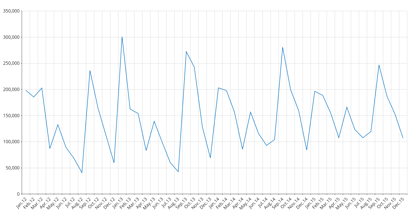
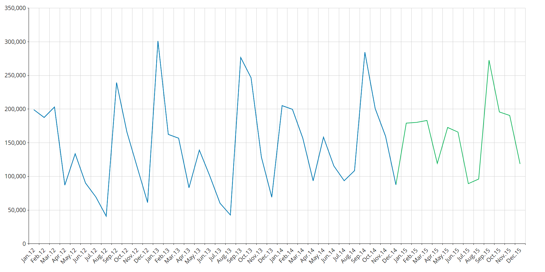
In the picture below you can see an example of historical data (in blue) forecasted to the future through the Predictive Analytics functionality (in green).
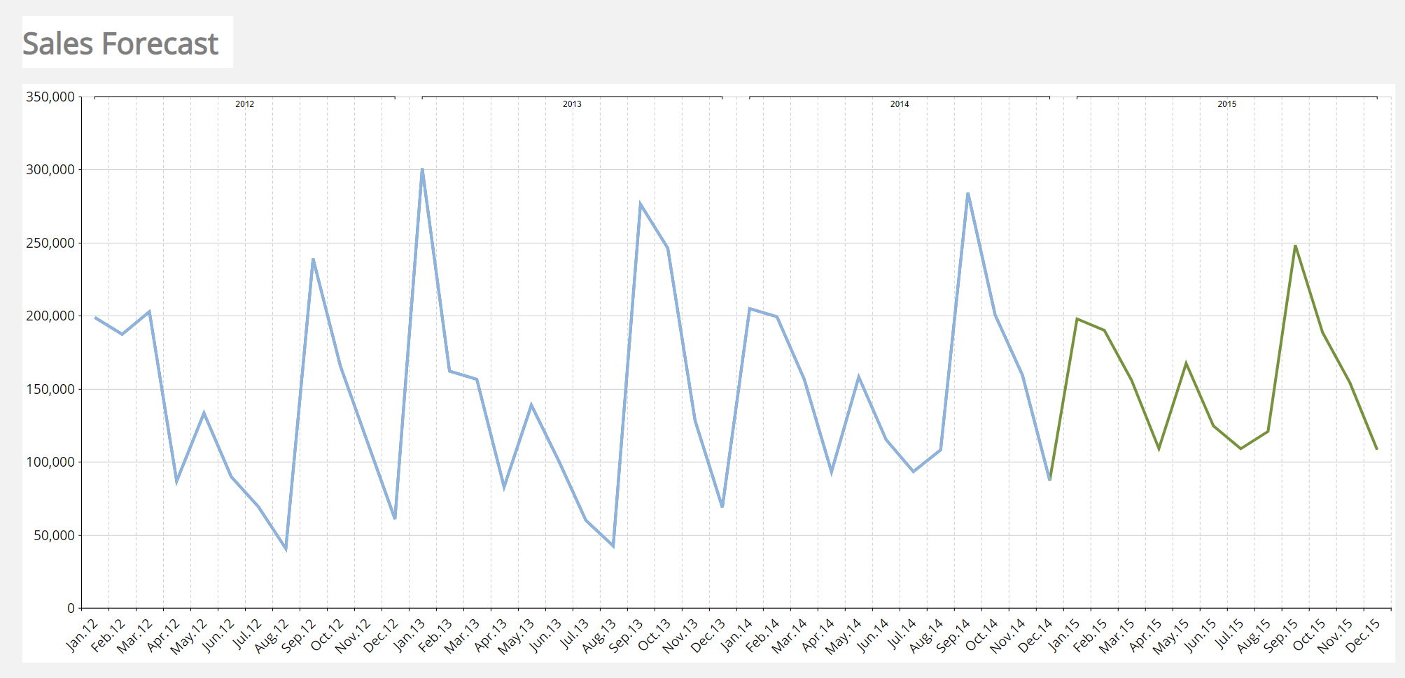
The Predictive Analytics tool is automatic in nature, but it is also very flexible as it allows you to refine its forecast by including additional information to the forecast scenarios: in fact, in addition to the historical time series, the user can feed the B.E.A.M. with other measures and parameters (covariates) that influence the forecast calculation. The B.E.A.M. determines which is the best model to be applied to historical data (learning phase), and then applies the defined model to future time periods (forecast phase).
How the Predictive Analytics scenario works
When you run a Predictive Analytics scenario based on one or multiple source Cubes, the Predictive Engine will:
- Detect the time series
- Label each time series as Discontinued, Intermittent or Smooth
- Trim the time series removing zero values at the beginning of each series
- Identify the best model for each series through competition
- Identify outliers
- Detect useful covariates, apply exogenous covariates and discards covariates that do not improve the model
- Serialize the model for future reuse
The process above is the the learning phase. Once it's completed, the system applies the model to future values (forecast horizon) and outputs various indicators: this part is the forecast phase.
See the following paragraphs for more details about the phases and concepts mentioned above (time series, outliers, covariates, etc.).
This whole process is automatic and the user has no perception of what is happening in the background. The user will be notified when the outputs of the process are ready.
Time series
Generally speaking, a time series is a series of values ordered in time (the so called Time Entities in Board, such as Day, Week, Month, etc.).
Example
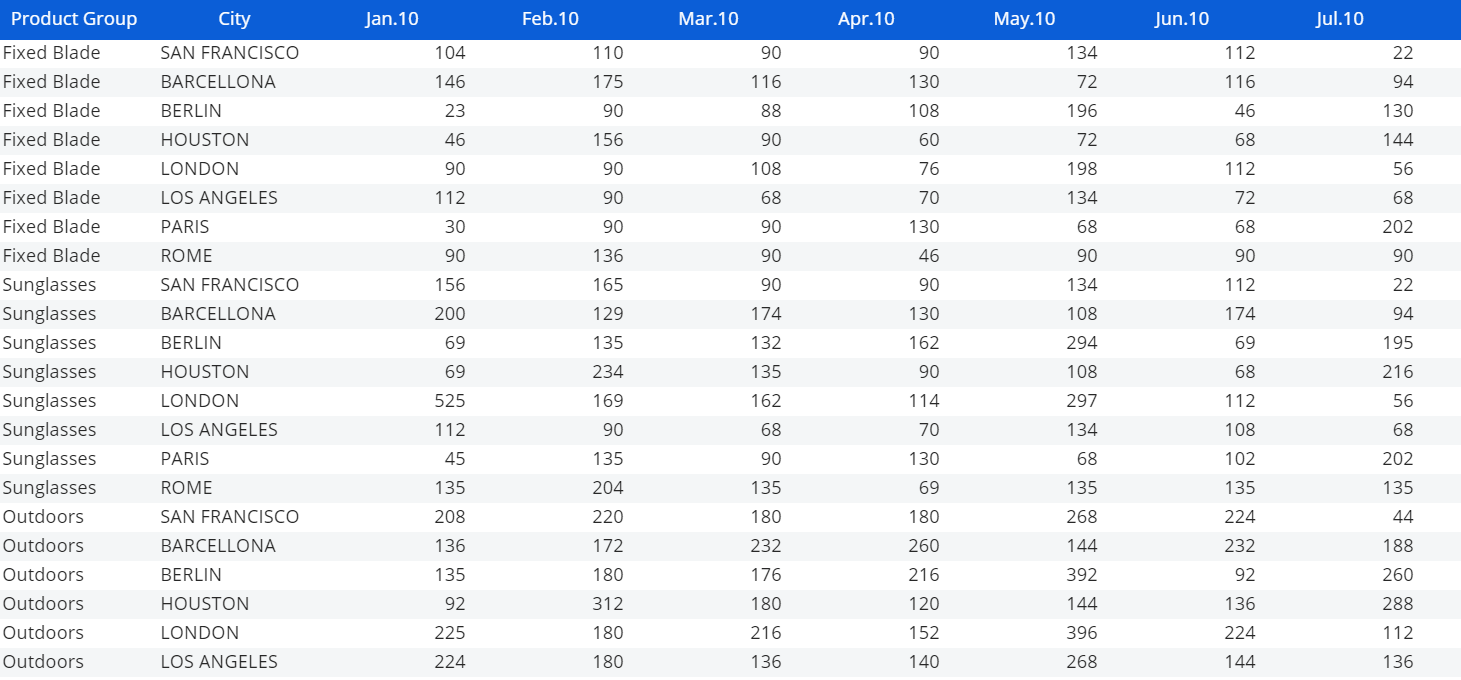
If you want to forecast data that is contained in a Cube (called, the observed Cube) structured by City, Product and Month, but you want to obtain the forecasted data at the Region, Product Group and Month level (i.e. the structure of the target Cube), in this case the time series is made of all the non-zero combinations of Region and Product Group in the source Cube.
The evaluation of the formulas is always done at the aggregation level of the target Cube.
| Entities in the Cube structure | Observed Cube | Target Cube |
| Month | X | X |
| Product | X | |
| Product Group | X | |
| Region | X | |
| City | X |
In other words, if in a Layout associated with a Data View you set Product Group and City By Row, and Month by Column, each row of the resulting Data View will represent a time series.
The number of time series is also called granularity.
Time series labeling
B.E.A.M. supports three types of labeling for time series data:
- Discontinued
- Intermittent
- Smooth.
Discontinued
A time series is discontinued if it’s definitively zero (data of the last year is always zero).
Intermittent
A time series is intermittent if it’s often zero but has values in some periods. For example, if you sell large machinery, you are unlikely to sell some every month, but you will most likely sell a few twice a year. A series like this can be labeled as intermittent.
To label a time series data as intermittent, the median elapsed time (in periods) between two non-zero values of the series is calculated: if this value is greater than 1.3 then the series is intermittent.
Smooth
A time series with values in every period is defined as smooth. Basically, all the series that are not intermittent or discontinued are smooth, that is, the median elapsed time (in periods) between two non-zero values of the series is less than 1.3.
Models
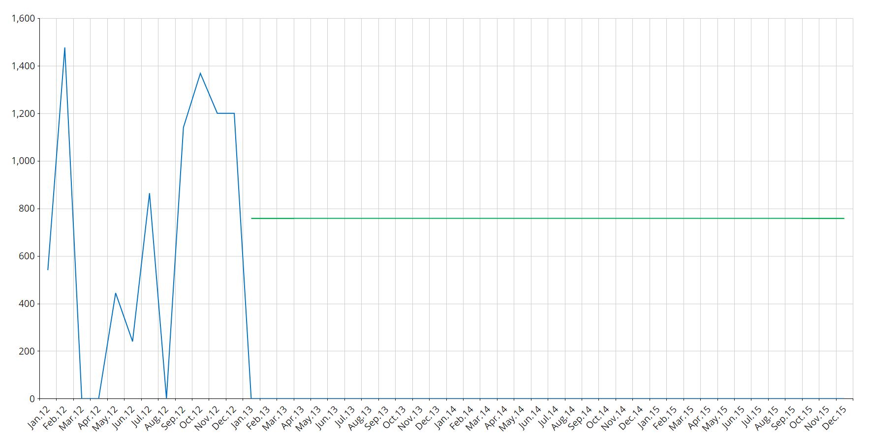
Discontinued time series are assumed to be zero also in the future, so the model for this type of series is simply a zero value on every period.
The Croston-SBA model will be used to forecast intermittent time series. Due to the nature of this model, the forecast for the future will be a constant for every period.
When it comes to smooth series, the scenario becomes a bit more complex. The model for time series is named Idsi-ARX and is part of the ARIMA (autoregressive integrated moving average) family. The ARIMA model is fitted to the time series through competition: the series is truncated into two parts at 0.75% of its length in periods, and the first part is used to calculate the ARIMA while the remaining part is used as a benchmark. Then, the model that best fits the scenario will be selected.
In the competition we will also have the two naïve predictors, the persistent one (constantly the last value of the series) and the seasonal one (basically a previous year). The model that wins the competition is chosen and used to calculate future values as well, using all data as input.
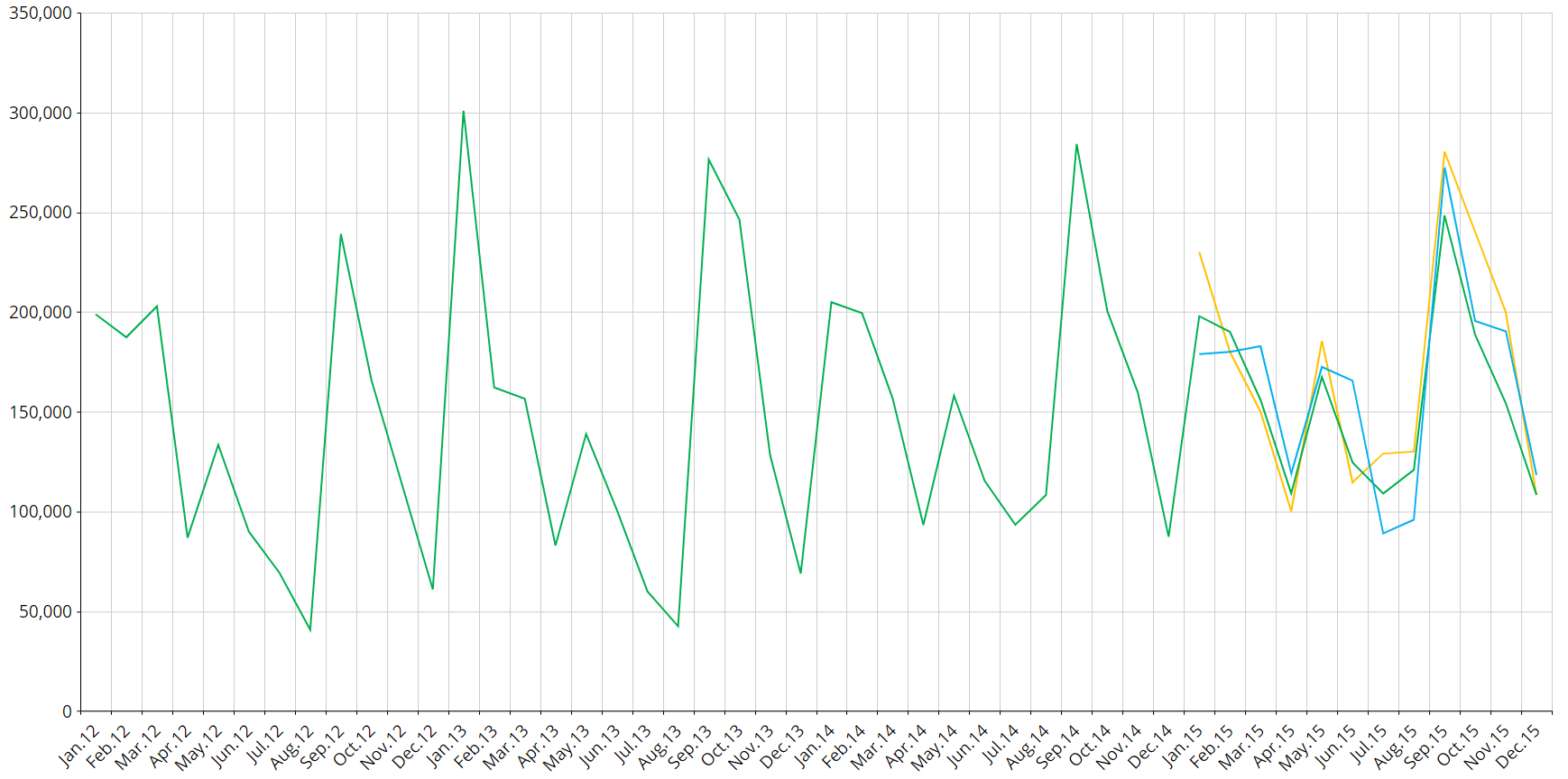
The picture below shows the concept of competition: the green series is predicted with orange and blue series, the blue is closer (in the squared error mean) to the original series, so it’s chosen versus the orange one.
Once the model is chosen, forecasts are calculated by adopting that model.
Outliers
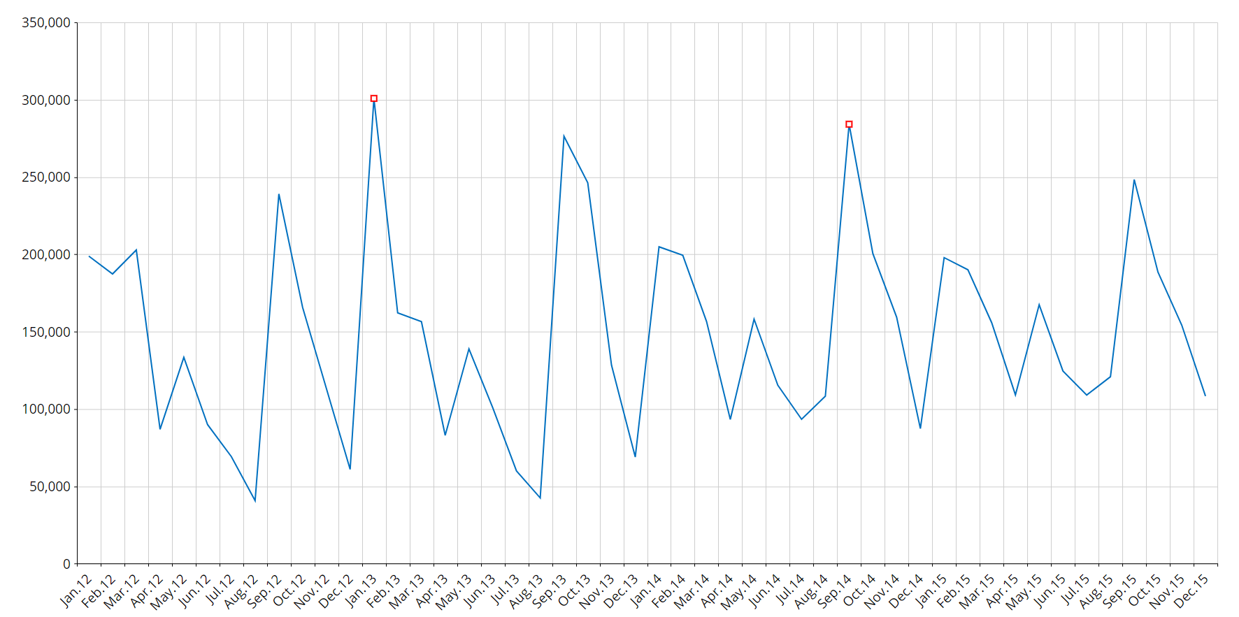
The system automatically detects anomalous values in the historic data: these data are called "outliers". A time series value is an outlier if its error against the model is more than 3.5 times the standard deviation.
In the image below, outliers are highlighted by red square markers.
Covariates
A covariate is a time series applicable to the entire time horizon (future and past) that is related to the observed time series.
For example, if you sell Easter eggs, a covariate would be a time series defined as 1 during the Easter period and 0 outside that same period.
The system evaluates the effect that this covariate had on the series and applies it to the future if and only if the covariate is significant: if the inclusion of the effect of the covariate in the prediction generates a bigger prediction error, the covariate is discarded.
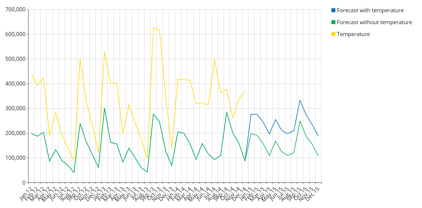
A covariate can be a boolean (like the sample's) or another time series (for example, the average temperature is a covariate when I am observing the ice creams sales time series).
It is not mandatory to set up future values for a covariate: for example, if you know that your store was closed during a certain period and this won’t happen in the future, you can simply inform the system that something out of the ordinary happened during that period and it will not happen again.
Example 1:
Forecast of Ice creams sales with and without the temperature covariate (forecast period is the 2015).
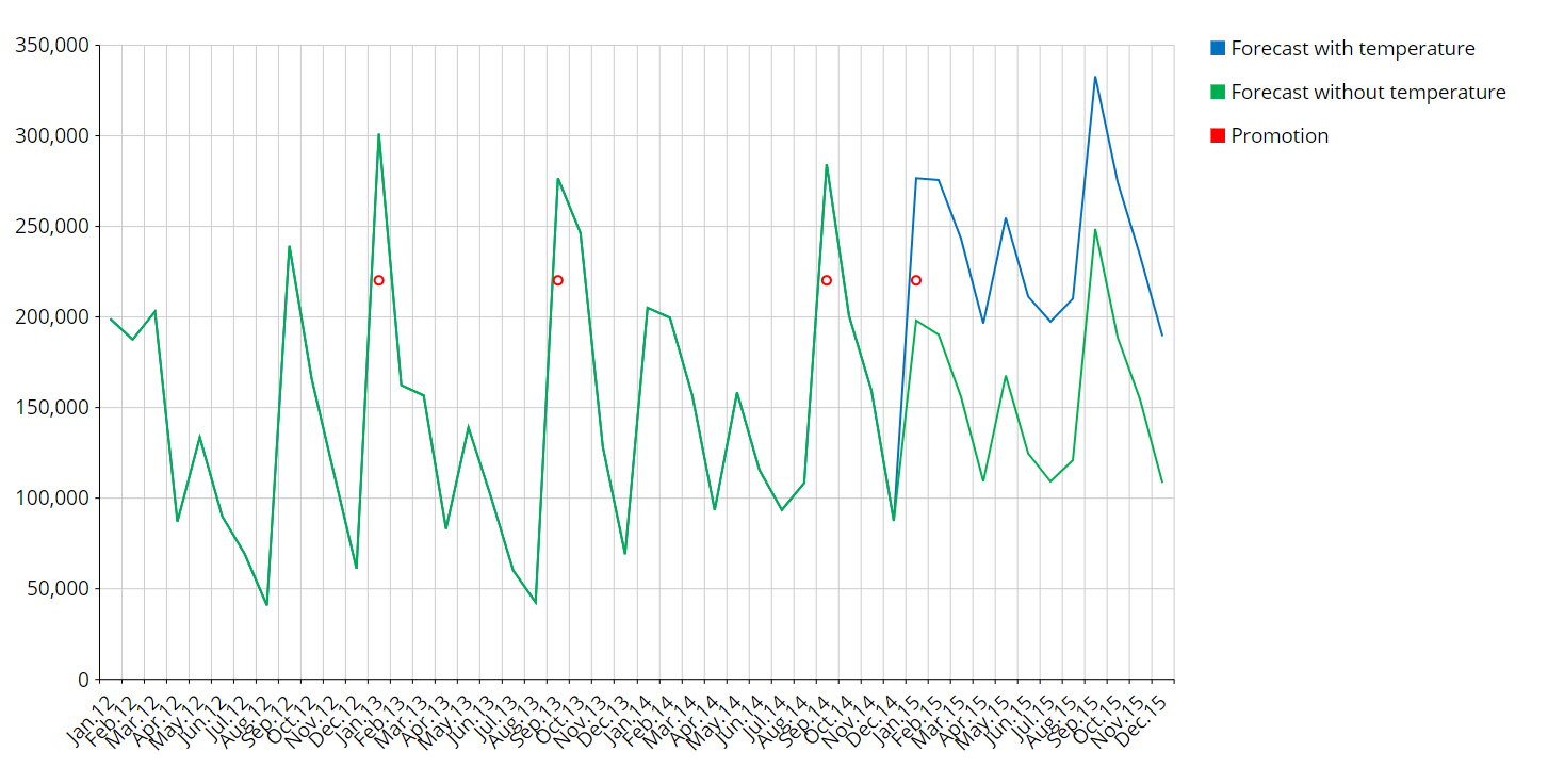
Example 2:
Promotion Campaigns for ice creams during some particular period (Past and Future Boolean Covariate, forecast period is 2015)
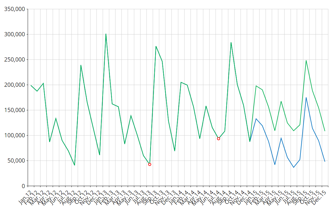
Example 3:
My ice cream shop closed twice in the past for a whole month, but I don't expect this to happen anymore (Past Boolean Covariate). The green series considers the covariate, blue series does not.
You can apply as many covariates as needed.
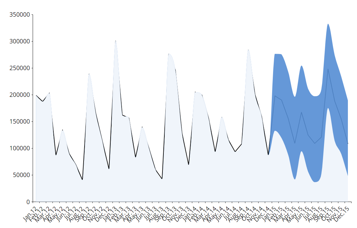
Prediction intervals
Given a level of confidence "X", a prediction interval is made of a certain number of periods of values where predicted values will fall with probability "X".
In other words, if we set a level of confidence of 90%, the system will provide a lower value and an higher value for the forecasted periods. Future observed values will fall between the low and high threshold with a 90% probability.
EXAMPLE:
At the end of 2015 we will observe that 90% of the values have fallen in the blue area of the graph below (forecast period is 2015).
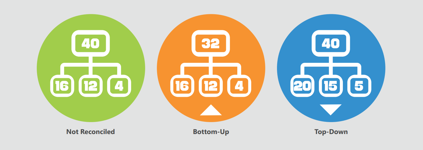
Reconciliation
When you have Cubes with multiple versions, B.E.A.M. will handle them considering each version as a separate scenario.
The sum of the forecasts of the more detailed versions is different from the forecast of the less detailed ones and this means that the target Cube is not aligned. You can choose not to align this Cube or to perform a reconciliation.
Two types of reconciliations are available: top-down and bottom-up.
- The top-down approach allocates data of the aggregated version to the most detailed version (similar to what happens with the split and splat feature), always respecting the existing proportions.
- The bottom-up approach aligns the data in the target Cube with the sum of the most detailed versions by aggregation.
Error statistics
The system supports the following machine learning metrics for regression models:
- MAE (Mean Absolute Error): it is the mean absolute difference between the actual and the predicted value. This measure is scale-dependent
- MAPE (Mean Absolute Percentage Error): it is the mean absolute percentage difference between the actual and the predicted value. This measure is not scale-dependent
- MASE (Mean Absolute Scaled Error): It’s the ratio of the MAE and the MAE of the naïve model. It is not scale-dependent and it measures the quality of forecast compared to the naïve forecast. A MASE grater than 1 indicates that the selected model performed worse than the naïve, while a MASE lower than 1 indicates that the selected model performed better than the naïve
- Weighted MASE Overall: This measure is the weighted average of all the MASE indicators of the various time series.